To set the scene, suppose we have a model with weights \(w\) and some loss function \(L(w)\) that we want to minimize. Then our objective is to find \(w^*\) where:
\[w^* = \underset{w}{\text{argmin}} L(w)\]Suppose we want to minimize how much our weights change between optimization iterations.
To do this, with \(w^{(k)}\) denoting the weights at the \(k\)-th iteration, we can add another term to our loss function \(\rho(w^{(k)}, w^{(k+1)})\) which minimizes how much the weights change between iterations like so:
\[w^{(k+1)} = \text{prox}_{L, \lambda}(w^{(k)}) = \underset{w^{(k+1)}}{\text{argmin}} [ L(w^{(k+1)}) + \lambda \rho(w^{(k)}, w^{(k+1)}) ]\]where \(\lambda\) controls how much the weights change between iterations (i.e larger \(\lambda\) = less change). This is called a proximal optimization method.
Most of this post is created in reference to Roger Grosse’s ‘Neural Net Training Dynamics’ course. The course can be found here and I would highly recommend checking it out. Though there are no lecture recordings, the course notes are in a league of their own.
Euclidean Space
For example, in Euclidean space we could define \(\rho\) to be the 2-norm between our weights:
\[\rho(w^{(k+1)}, w^{(k)}) = \dfrac{1}{2} \| w^{(k+1)} - w^{(k)}\|^2\]And so we would get:
\[w^{(k+1)} = \text{prox}_{L, \lambda}(w^{(k)}) = \underset{w^{(k+1)}}{\text{argmin}} [ L(w^{(k+1)}) + \lambda \dfrac{1}{2} \|w^{(k+1)} - w^{(k)}\|^2 ]\]Lets try to solve for the optimum (i.e \(w^{(k+1)} = w^*\)) by computing the grad and setting it = 0:
\[\begin{align*} 0 &= \nabla L(w^*) + \lambda (w^* - w^{(k)}) \\ - \lambda^{-1} \nabla L(w^*) &= (w^* - w^{(k)}) \\ w^* &= w^{(k)} - \lambda^{-1} \nabla L(w^*) \\ \end{align*}\]The equation looks very similar to SGD however, \(\nabla L\) is defined at \(w^*\), which we don’t know, so we can’t directly use this result.
Although we can’t use this result directly, there are a few approximations we could use to make the result useful…
First Order Approximation of \(L\) around \(w^{(k)}\)
Note: For the following sections it would be good to be comfortable with Taylor series approximations. If you aren’t, I would recommend grabbing a cup of tea and enjoy 3b1b’s video on the topic.
One possible way to use the result is to approximate \(L(w^{(k+1)})\) with a first-order Taylor series around \(w^{(k)}\):
\[L(w^{(k+1)}) = L(w^{(k)}) + \nabla L(w^{(k)})^\intercal(w^{(k+1)} - w^{(k)})\]Substituting this into our loss we get:
\[\begin{align*} \text{prox}_{L, \lambda}(w^{(k)}) =& \underset{w^{(k+1)}}{\text{argmin}} [ L(w^{(k+1)}) + \lambda \rho(w^{(k+1)}, w^{(k)}) ] \\ \approx& \underset{w^{(k+1)}}{\text{argmin}} [ L(w^{(k)}) + \nabla L(w^{(k)})^\intercal(w^{(k+1)} - w^{(k)}) + \lambda \rho(w^{(k+1)}, w^{(k)}) ] \\ =& \underset{w^{(k+1)}}{\text{argmin}} [\nabla L(w^{(k)})^\intercal w^{(k+1)} + \lambda \rho(w^{(k+1)}, w^{(k)}) ] \\ \end{align*}\]Note: we go from the second to the third line since \(\text{argmin}_{w^{(k+1)}}\) ignores any terms without \(w^{(k+1)}\).
Then similar to the previous section, we can solve for the optimum by computing the gradient and setting it = 0:
\[\begin{align*} 0 &= \nabla L(w^{(k)}) + \lambda (w^* - w^{(k)}) \\ w^* &= w^{(k)} - \lambda^{-1} \nabla L(w^{(k)}) \\ \end{align*}\]The result is standard gradient descent!
Notice how if we want our weights to be very close together across iterations then we would set \(\lambda\) to be a large value so \(\lambda^{-1}\) would be a small value and so we would be taking very small gradient steps to reduce large changes in our weights across iterations.
This means that in Euclidean space:
- proximal optimization approximated with a first-order Taylor is the same as regular gradient descent.
Use a Second-Order Approximation of \(\rho\)
Another way we could solve the equation is to use the first-order approximation of \(L\) with a second-order approximation of \(\rho\). Furthermore, we would let \(\lambda \rightarrow \infty\) (we want our steps to be as close as possible).
Note: Though we don’t need to do this since we solved it directly in the last section, the ideas in this simple example will complement the rest of the post nicely.
To compute our second order approximation of \(\rho\) we need to compute \(\nabla \rho\) and \(\nabla^2 \rho\).
To do so, we take advantage of the fact \(\lambda \rightarrow \infty\). This implies that in Euclidean space, \(w^{(k+1)} \approx w^{(k)}\). And so we get:
\[\rho (w^{(k+1)}, w^{(k)}) = \dfrac{1}{2} \|w^{(k)} - w^{(k+1)} \|^2 \approx \dfrac{1}{2} \|w^{(k)} - w^{(k)} \|^2 = 0\]…
\[\nabla \rho (w^{(k+1)}, w^{(k)}) = (w^{(k)} - w^{(k+1)}) \approx (w^{(k)} - w^{(k)}) = 0\]…
\[\nabla^2 \rho (w^{(k+1)}, w^{(k)}) = 1\]Since both \(\rho\) and \(\nabla \rho\) are both \(0\) when we approx \(\rho\) with a second-order Taylor series, we are left with only our second order approximation (\(\nabla^2 \rho = G = \text{I}\)):
\[\begin{align*} \rho (w^{(k+1)}, w^{(k)}) &\approx \rho(w^{(k+1)}, w^{(k)}) + \nabla \rho(w^{(k+1)}, w^{(k)})^\intercal (w^{(k+1)} - w^{(k)}) + \dfrac{1}{2} (w^{(k+1)} - w^{(k)})^\intercal G (w^{(k+1)} - w^{(k)}) \\ &= \dfrac{1}{2} (w^{(k+1)} - w^{(k)})^\intercal G (w^{(k+1)} - w^{(k)}) \end{align*}\]Using the second-order approx of \(\rho\) with the first-order approx of \(L\) which we derived in the last section we get the following loss function:
\[\begin{align*} \text{prox}_{L, \lambda}(w^{(k)}) =& \underset{w^{(k+1)}}{\text{argmin}} [ L(w^{(k+1)}) + \lambda \rho(w^{(k)}, w^{(k+1)}) ] \\ \approx& \underset{w^{(k+1)}}{\text{argmin}} [\nabla L(w^{(k)})^\intercal w^{(k+1)} + \lambda \dfrac{1}{2} (w^{(k+1)} - w^{(k)})^\intercal G (w^{(k+1)} - w^{(k)})] \end{align*}\]Solving for the optimal \(w^*\) we get:
\[\begin{align*} w^* &= w^{(k)} - \lambda^{-1} \text{G}^{-1} \nabla L(w^{(k)}) \end{align*}\]In Euclidean space \(\text{G} = \nabla^2 \rho (w^{(k+1)}, w^{(k)}) = \text{I}\), so again we get gradient descent:
\[\begin{align*} w^* &= w^{(k)} - \lambda^{-1} \text{G}^{-1} \nabla L(w^{(k)}) \\ &= w^{(k)} - \lambda^{-1} \text{I}^{-1} \nabla L(w^{(k)}) \\ &= w^{(k)} - \lambda^{-1} \nabla L(w^{(k)}) \end{align*}\]Though this doesn’t conclude anything new compared to the previous section, this shows how we can use a second-order approximation for \(\rho\) to derive an update rule.
KL Divergence
Now, Euclidean space is great, but sometimes Euclidean space isn’t always that great:
Why KL? Ex 1
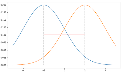
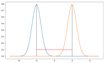
In the two images, we see two Gaussians (coloured orange and blue)(example taken from here).
If we parameterize the Gaussians by their parameters (i.e their mean value \(\mu\)) then both examples have the same Euclidean distance between them (shown in red). This is called parameter space. However, we see that the distributions in the first image are much closer than the ones in the second.
Ideally, we would want a smaller metric for the first image than the second image.
To achieve this, a better measurement would be to use the KL-Divergence between the distributions. This measures the distance in distribution space.
Why KL? Ex 2
Another reason we may prefer KL Divergence over Euclidean distance is that it minimizes the change of our model’s output directly. For example, if we were to only minimize the change of our weights, a small change in our weights may lead to a large difference in our model’s predictions which we wouldn’t want.
KL
More formally, KL-Divergence (\(D_{KL}\)) measures the distance between two distributions \(p(x \vert \theta')\) and \(p(x \vert \theta)\) which are parameterized by \(\theta'\) and \(\theta\) and is defined as:
\[\begin{align*} D_{KL}[p(x \vert \theta) \| p(x \vert \theta')] &= \sum_x p(x|\theta) [\log \dfrac{p(x \vert \theta)}{p(x \vert \theta')}] \\ &= \sum_x p(x|\theta) [\log p(x \vert \theta) - \log p(x \vert \theta')] \\ &= \mathbb{E}_{p(x \vert \theta)} [\log p(x \vert \theta) - \log p(x \vert \theta')] \\ \end{align*}\]Note: \(D_{KL}\) cannot be applied to neural networks with weights \(w\) because it measures the distance between distributions, which \(w\) is not. To show this difference we will let \(\theta^{(k)}\) parameterize some distribution \(p(x \vert \theta^{(k)})\) at the \(k\)-th step of optimization.
Teaser: We’ll see how to apply this to neural nets later ;)
Lets assume were minimizing a loss function \(L\) parameterized by \(\theta\) and that we want \(\theta^{(k)}\) and \(\theta^{(k+1)}\) to be close across steps. Then we can let \(\rho(\theta^{(k)}, \theta^{(k+1)}) = D_{KL}(p_{\theta^{(k)}} \| p_{\theta^{(k+1)}})\) where \(p_{\theta^{(k)}} = p(x \vert \theta^{(k)})\). And so, we will want to solve for:
\[\begin{align*} \theta^* = \text{prox}_{L, \lambda}(\theta^{(k)}) =& \underset{\theta^{(k+1)}}{\text{argmin}} [ L(\theta^{(k+1)}) + \lambda \rho(\theta^{(k)}, \theta^{(k+1)}) ] \\ =& \underset{\theta^{(k+1)}}{\text{argmin}} [ L(\theta^{(k+1)}) + \lambda D_{KL}(p_{\theta^{(k)}} \| p_{\theta^{(k+1)}}) ] \\ \end{align*}\]\(\nabla D_{KL}\) and \(\nabla^2 D_{KL}\)
Similar to last section, lets fisrt approximate \(D_{KL}(p_{\theta^{(k)}} \| p_{\theta^{(k+1)}})\) with a second-order taylor expansion. Recall from the previous section to approximate \(\rho\) with a second-order taylor series we need to define \(\rho\vert_{\theta'=\theta}\), \(\nabla \rho\vert_{\theta'=\theta}\) and \(\nabla^2 \rho\vert_{\theta'=\theta}\).
First, lets derive \(\rho\), \(\nabla \rho\), and \(\nabla^2 \rho\) for \(D_{KL}\)
\[\begin{align*} \rho = D_{KL}[p(x \vert \theta) \| p(x \vert \theta')] &= \mathbb{E}_{p(x \vert \theta)} [\log p(x \vert \theta) - \log p(x \vert \theta')] \\ &= \mathbb{E}_{p(x \vert \theta)} [\log p(x \vert \theta)] - \mathbb{E}_{p(x \vert \theta)}[\log p(x \vert \theta')] \\ \end{align*}\]…
\[\begin{align*} \nabla \rho = \nabla_{\theta'} D_{KL}[p(x \vert \theta) \| p(x \vert \theta')] &= \nabla_{\theta'} \mathbb{E}_{p(x \vert \theta)} [\log p(x \vert \theta)] - \nabla_{\theta'} \mathbb{E}_{p(x \vert \theta)}[\log p(x \vert \theta')] \\ &= - \nabla_{\theta'} \mathbb{E}_{p(x \vert \theta)}[\log p(x \vert \theta')] \\ &= - \nabla_{\theta'} \int p(x \vert \theta) \log p(x \vert \theta') \text{d}x \\ &= - \int p(x \vert \theta) \nabla_{\theta'} \log p(x \vert \theta') \text{d}x \end{align*}\]…
\[\begin{align*} \nabla^2 \rho = \nabla_{\theta'}^2 D_{KL}[p(x \vert \theta) \| p(x \vert \theta')] &= - \int p(x \vert \theta) \nabla_{\theta'}^2 \log p(x \vert \theta') \text{d}x \\ \end{align*}\]To evaluate \(\rho\vert_{\theta'=\theta}\), \(\nabla \rho\vert_{\theta'=\theta}\) and \(\nabla^2 \rho \vert_{\theta'=\theta}\) we are going to need the two following equations:
\[\mathbb{E}_{p(x|\theta)} [\nabla_{\theta} \log p(x \vert \theta)] = 0\]and
\[\mathbb{E}_{p(x|\theta)} [ \nabla_{\theta}^2 \log p(x \vert \theta) ] = -\text{F}\]Where \(\text{F} = \mathop{\mathbb{E}}_{p(x \vert \theta)} \left[ \nabla \log p(x \vert \theta) \, \nabla \log p(x \vert \theta)^{\text{T}} \right]\) is the fisher information matrix. For the full derivation of these equations checkout this blog post.
And so using these equations, we get:
\[\begin{align*} \nabla_{\theta'} D_{KL}[p(x \vert \theta) \| p(x \vert \theta')] |_{\theta' = \theta} &= - \int p(x \vert \theta) \nabla_{\theta'} \log p(x \vert \theta')|_{\theta' = \theta} \text{d}x \\ &= - \mathbb{E}_{p(x|\theta)} [\nabla_{\theta} \log p(x \vert \theta)] \\ &= 0 \end{align*}\] \[\begin{align*} \nabla_{\theta'}^2 D_{KL}[p(x \vert \theta) \| p(x \vert \theta')] |_{\theta' = \theta} &= - \int p(x \vert \theta) \nabla_{\theta'}^2 \log p(x \vert \theta') |_{\theta' = \theta} \text{d}x \\ &= - \mathbb{E}_{p(x|\theta)} [ \nabla_{\theta}^2 \log p(x \vert \theta) ] \\ &= \text{F} \\ \end{align*}\]Then using the first-order approximation of \(L\) with our second-order approximation of \(D_{KL}\) we get:
\[\begin{align*} \text{prox}_{L, \lambda}(\theta^{(k)}) =& \underset{\theta^{(k+1)}}{\text{argmin}} [ L(\theta^{(k+1)}) + \lambda D_{KL}(p_{\theta^{(k)}} \| p_{\theta^{(k+1)}}) ] \\ \approx& \underset{\theta^{(k+1)}}{\text{argmin}} [\nabla L(\theta^{(k)})^\intercal \theta^{(k+1)} + \lambda \dfrac{1}{2} (\theta^{(k+1)} - \theta^{(k)})^\intercal F (\theta^{(k+1)} - \theta^{(k)})] \\ \end{align*}\]Computing the gradient and setting it to zero we get
\[\begin{align*} \theta^* &= \theta^{(k)} - \lambda^{-1}\text{F}^{-1}\nabla L(\theta^k) \\ \end{align*}\]This update rule is called natural gradient descent. Fantastic!
Now you’re probably thinking:
“Indeed, this is fantastic, we now know how to constrain distributions across iterations using \(D_{KL}\) but how do we apply it to neural networks with weights \(w\)??”
Excellent question, let’s check it out in the next section
Natural Gradient Descent for Neural Nets
Though our weights \(w\) aren’t a distribution, usually, our model outputs a distribution \(r( \cdot \vert x)\). For example, in classification problems like MNIST our model’s outputs a probability distribution over the digits 1 - 10 (\(p( y \vert x)\)).
The idea is that even though we can’t constrain our weights across iterations with \(D_{KL}\), we can use \(D_{KL}\) to constrain the difference between our output distributions across iterations which is likely to do something similar.
Decomposition Trick
To do this, we need to use a trick. Specifically, we need to decompose \(\rho\) into two parts:
- Network forward pass: \(z = f(w, x)\) where \(z\) is a probability distribution
- Distribution Distance: \(\rho(z_0, z_1) = D_{KL}(z_0, z_1)\) computation for some $z_0$ and $z_1$
Then we can define the full \(\rho_{\text{pull}}\) as the composition of the two parts:
\[\rho_{\text{pull}} = \rho(f(w^{(k)}, x), f(w^{(k+1)}, x))\]\(\rho_{\text{pull}}\) and \(\nabla \rho_{\text{pull}}\)
Now similar to the previous sections, lets approximate \(\rho_{\text{pull}}\) with a second-order Taylor expansion. Again, we need to find \(\rho_{\text{pull}}(w, w')\vert_{w = w'}\), \(\nabla \rho_{\text{pull}}(w, w')\vert_{w = w'}\), and \(\nabla_{\text{pull}}^2 \rho(w, w')\vert_{w = w'}\):
\[\begin{align*} \rho_{\text{pull}}(w, w')\vert_{w = w'} &= \rho(f(w', x), f(w', x)) \\ &= 0 \\ \end{align*}\]…
\[\begin{align*} \nabla_w \rho_{\text{pull}}(w, w')\vert_{w = w'} &= \nabla_w\rho(f(w, x), f(w', x)) \\ &= \text{J}_{zx}^\intercal \underbrace{\nabla_z\rho(z, z')|_{z=z'}}_{=0} \\ &= 0 \\ \end{align*}\]We derive the last line by using the chain rule and the fact that \(\nabla \rho = \nabla D_{KL} = 0\) (derived in the previous section).
Now to show the power of the two-part decomposition we used…
Decomposing \(\nabla^2 \rho_{\text{pull}}\) – The Guass-Newton Hessian
Using the two-part decomposition it can be shown that \(\nabla^2 \rho_{\text{pull}}\) (in general any hessian/second derivative matrix) can be represented as the following (check out this for a full derivation):
\[\begin{align*} \nabla_w^2 \rho_{\text{pull}}(w, w') &= \text{J}_{zw}^\intercal H_z \text{J}_{zw} + \sum_a \dfrac{d \rho}{dz_a} \nabla^2_w [f(x, w)]_a\\ \end{align*}\]Now let’s better understand what this representation means. This shows that $\nabla_w^2 \rho_{\text{pull}}(w, w’)$ can be represented as two parts:
\[\text{J}_{zw}^\intercal H_z \text{J}_{zw}\]- First derivatives of the network (i.e, $\text{J}_{zw}$ the Jacobian of $\dfrac{dz}{dw}$) and second derivatives of $\rho$ (i.e, $H_z$)
- Second derivaties of the network (i.e, $\nabla^2_w [f(x, w)]_a$) and first derivatives of $\rho$ (i.e, $\dfrac{d \rho}{dz_a}$)
Usually computing and storing second derivatives of the network is very expensive (for a network with $n$ parameters the second derivative matrix will be of size $n \times n$ where $n$ is usually in millions for neural networks). Luckily though, since we know \(\nabla \rho = \nabla D_{KL} = 0\) we drop the second derivatives:
\[\begin{align*} \nabla_w^2 \rho_{\text{pull}}(w, w') &= \text{J}_{zw}^\intercal H_z \text{J}_{zw} + \underbrace{\sum_a \overbrace{\dfrac{d \rho}{dz_a}}^{=0} \nabla^2_w [f(x, w)]_a}_{=0} \\ &= \text{J}_{zw}^\intercal H_z \text{J}_{zw} \end{align*}\]Note: When \(\nabla \rho \neq 0\) we can approximate \(\nabla_w^2 \rho_{\text{pull}}\) by just setting \(\nabla \rho = 0\), using \(\text{J}_{zw}^\intercal H_z \text{J}_{zw}\) and hope for the best lol. This formulation is called the Guass-Newton Hessian. In this case though ($\rho = D_{KL}$), the Guass-Newton Hessian is the exact solution.
Natural Gradient Descent
In the previous section we derived that \(\nabla^2 \rho = \nabla^2 D_{KL} = H_z = F_z\) where \(F_z\) is the fisher information matrix. And so using the definition of the fisher matrix (i.e \(\text{F} = \mathop{\mathbb{E}}_{p(x \vert \theta)} \left[ \nabla \log p(x \vert \theta) \, \nabla \log p(x \vert \theta)^{\text{T}} \right]\)) with our networks output we can derive our second-order approximation:
\[\begin{align*} \nabla_w^2 \rho_{\text{pull}}(w, w') &= \mathbb{E_{x \sim p_{\text{data}}}} [\text{J}_{zw}^\intercal \text{F}_z \text{J}_{zw}] \\ &= \mathbb{E_{x \sim p_{\text{data}}}} [\text{J}_{zw}^\intercal \mathbb{E}_{t \sim r(\cdot \vert x)} [\nabla_z \log r(t \vert x) \nabla_z \log r(t \vert x) ^ \intercal] \text{J}_{zw}] \\ &= \mathbb{E_{x \sim p_{\text{data}}, {t \sim r(\cdot \vert x)}}} [\nabla_w \log r(t \vert x) \nabla_w \log r(t \vert x) ^ \intercal] \\ &= \text{F}_w \end{align*}\]Notice \({t \sim r(\cdot \vert x)}\) samples \(t\) from the model’s distribution which is the true fisher information matrix.
Similar, but not the same, is the empirical fisher information matrix where \(t\) is taken to be the true target.
In total, using our approximation we get the following second-order approximation:
\[\rho_{\text{pull}}(w, w') \approx \dfrac{1}{2} (w - w')^\intercal \text{F}_w (w - w')\]Which again, if we compute the gradient and set it to zero, we get:
\[\begin{align*} w^{(k+1)} &= \underset{w^{(k+1)}}{\text{argmin}} [\nabla L(w^{(k)})^\intercal w^{(k+1)} + \lambda \dfrac{1}{2} (w^{(k)} - w^{(k+1)})^\intercal \text{F}_w (w^{(k)} - w^{(k+1)})] \\ 0 &= \nabla L(w^{(k)}) + \lambda (w^{(k)} - w^*)^\intercal \text{F}_w \\ - \lambda^{-1} \text{F}_w^{-1}\nabla L(w^{(k)}) &= (w^{(k)} - w^*) \\ w^* &= w^{(k)} - \lambda^{-1} \text{F}_w^{-1}\nabla L(w^{(k)}) \\ \end{align*}\]We now see that this results in the natural gradient method for neural networks :D
Computing the Natural Gradient in JAX
The theory is amazing but it doesn’t mean much if we can’t use it. So, to finish it off we’re gonna code it!
To do so, we’ll write the code in JAX (what all the cool kids are using nowadays) and train a small MLP model on the MNIST dataset.
If you’re new to JAX there’s a lot of great resources out there to learn from! Specifically, make sure you’re comfortable with jax.jvp and jax.vjp to understand the code:
jax.jvp:lambda v:\(J v\)- Short Explanation: Jacobian vector product using reverse/backward-accumulation (
v.shape= output size)
- Short Explanation: Jacobian vector product using reverse/backward-accumulation (
jax.vjp:lambda v:\(v^T J\)- Short Explanation: Jacobian vector product using forward-accumulation (
v.shape= input size)
- Short Explanation: Jacobian vector product using forward-accumulation (
The full code can be found here.
Implementation: Common Gotchas and Programming Tricks
To implement the natural gradient here are a few pseudosteps:
- Compute gradients \(\nabla L(w)\)
- Construct the fisher information matrix \(\text{F}_w\)
- Compute \(\text{F}_w^{-1} \nabla L(w)\)
- Take a step: \(w^{(k+1)} = w^{(k)} - \lambda^{-1} \text{F}_w^{-1}\nabla L(w^{(k)})\)
Step 1 and 4 are easy; Step 2 and 3 are difficult. We will tackle how to implement steps 2 and 3 in the following section. The method we’ll use is called Hessian Free Optimization since we never explicitly represent the hessian matrix. However, there are many other methods to solve Step 2 and 3 (which may or may not be covered in an upcoming post…).
2. Construct the Fisher \(\text{F}_w\)
A straightforward implementation would construct the Fisher matrix explicitly like so:
- Compute the gradients \(\nabla L(w^{(k)})\) using autodiff and flatten/reshape them into a $n \times 1$ matrix
- Compute the fisher matrix \(F_w = \nabla L \nabla L^T\) as a $n \times n$ matrix
However, when \(n\) is large, we can’t compute the Fisher matrix explicitly since we have limited computer memory.
For example: A two layer MLP (with layers: 128 hidden and 10 output classes) for MNIST images (\(28 \times 28\) images -> \(784\) flattened image) consists of two weight matricies & some biases. Considering only the weight matricies: one with size \(754 \times 128\) and another \(128 \times 10\). This means the total number of parameters (\(n\)) is 96K (\(754 \times 128\)) + 1.2K (\(128 \times 10\)) = 97K. So constructing our fisher will be a \(97,000 \times 97,000\) matrix which is over 9 billion values. Try computing this and you’ll crash your macbook lol.
There are multiple ways around this problem but the one we will cover is matrix-vector products (MVP). We’ll see why soon.
3. Computing \(\text{F}_w^{-1} \nabla L(w)\)
Before we talk about matrix-vector products it makes sense to talk about how to compute \(\text{F}_w^{-1} \nabla L(w)\). To do so, we can use the conjugate gradient method. I won’t go in-depth on the algorithm (I left some resources at the end of the post) but all you need to know is that the method can approximately solve the following:
\[\underset{x}{\text{argmin}} \; A x = b\]For some matrices A, x, and b. For our problem, we can change the notation to:
\[\underset{x}{\text{argmin}} \; F_w x = \nabla L\]where \(\underset{x}{\text{argmin}} = F_w^{-1} \nabla L\), which is what we want. The best part is that the algorithm doesn’t require the full matrix \(F_w\) and only needs a way to compute the matrix-vector product \(F_w x\). Fortunately, there are ways to compute matrix-vector products without explicitly having the full matrix in memory.
Exercise: What’s the simplest way to compute an MVP without explicitly representing the full matrix in memory? See Conjugate Gradient resources for the answer.
2. + 3.: MVPs and Conjugate Gradient
Updating the pseudosteps we get:
- Compute gradients \(\nabla L(w)\)
- Define the MVP:
lambda v:\(\text{F}_w v\) - Compute \(\text{F}_w^{-1} \nabla L(w)\) using the conjugate gradient method and the MVP
- Take a step: \(w^{(k+1)} = w^{(k)} - \lambda^{-1} \text{F}_w^{-1}\nabla L(w^{(k)})\)
Jax: Setup
First, we define a small MLP model:
Then we define a few loss functions
Next, we make the losses work for batch input using vmap
Single example -> batch data with a single line? yes, please
To get a general feel for JAX, we first define a normal gradient step function (we use @jit to compile the function which makes it run fast)
Jax: 2. Define the MVP
We’ll use the equation above for comparison but we can also compute the Guass-Newton hessian:
Jax: Empirical Fisher
Note: Although we should be using the gradients from mean_log_likelihood, we can use the grads from the mean_cross_entropy to shave off an extra forward and backward pass. Exercise: Why does this work? (Hint: does fisher_vp change if we use nll vs ll?)
Jax: Natural Fisher
Speed Test
Results
| Optim Method | Test Accuracy (%) | Total Runtime (seconds) |
|---|---|---|
| Vanilla-SGD | 95.99 | 53 |
| Natural Gradient (Empirical) | 96.25 | 58 |
| Natural Gradient | 95.82 | 75 |
Further Reading and Brief Other Things
Problems with Inversion - Conjugate Gradient & Preconditioners
Problems when solving for $F^{-1} \nabla L$ – Conjugate Gradient Section – Stanford Lectures @ http://www.depthfirstlearning.com/2018/TRPO
Problems with Linearlizing
Recall: We linearize our solution with a Taylor-Approx and then solve for the optimal to take a step.
Problem: The optimal of the Taylor-Approx may not be the actual optimal. When the optimal is a large step away it may make the update even worse (see quick hand-drawn diagram below where we would end up at $\hat{f}_{optimal}$ which leads to a much worse value of $f(x)$ than our starting position $x$).
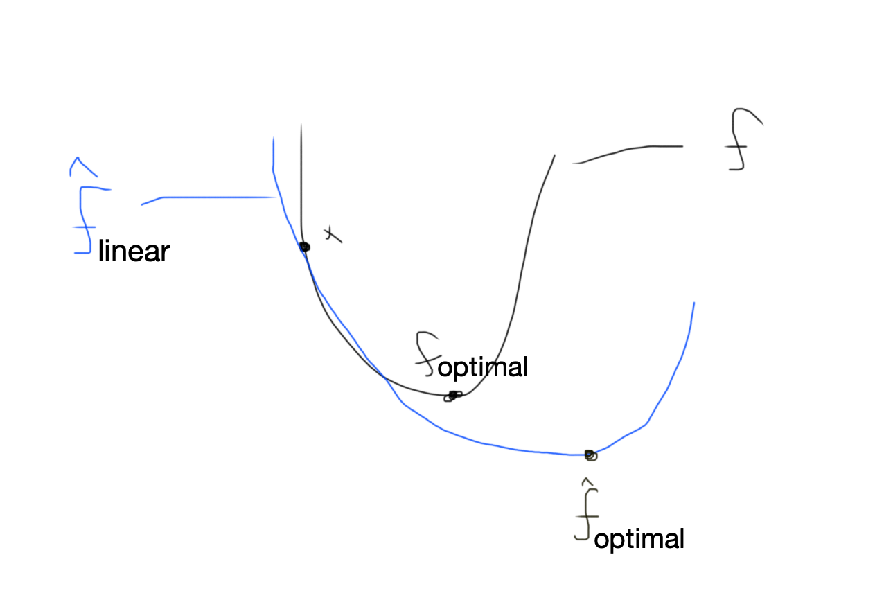
Soln: We can add another term \(\| w^{(k+1)} - w^{(k)}\|^2\) to our loss to make sure we don’t take large steps where our approximation is inaccurate. This leads to a dampened update:
Note: This is similar to Trust Region Optimization
More Resources
Cool conjugate gradient resource.
2nd-order Optimization for Neural Network Training from jmartens
https://www.cs.utoronto.ca/~jmartens/docs/HF_book_chapter.pdf