
Generative Adversarial Networks (GANs) have shown great results in computer vision but how do they perform when applied to time-series data? Following this, do Convolutional Neural Networks (CNNs) or do Recursive Neural Networks (RNNs) achieve the best results?
In this post, we discuss GAN implementations which aim to generate time-series data including, C-RNN-GANs (Mogren, 2016), RC-GANs (Esteban et al., 2017) and TimeGANs (Yoon et al., 2019). Lastly, we implement RC-GAN and generate stock data.
Basic GAN Intro
There are many great resources on GANs so I only provide an introduction here.
GANs include a generator and a discriminator. The generator takes latent variables as input (usually values sampled from a normal distribution) and outputs generated data. The discriminator takes the data (real or generated/fake) as input and learns to discriminate between the two.
The gradients of the discriminator are used both to improve the discriminator and improve the generator.
Here’s a nice picture for the more visually inclined from a wonderful blog.
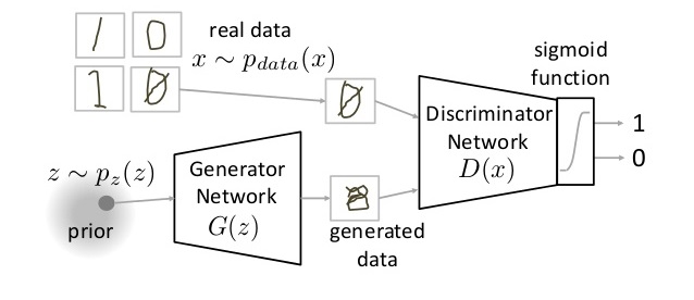
and a nice equation for the more equation-y inclined where \(D\) is the discriminator and \(G\) is the generator.
\[\min_G \max_D \mathbb{E}_{x\sim p_{data}(x)}[\log D(x)] + \mathbb{E}_{z\sim p_z(z)}[\log(1 - D(G(z)))]\]C-RNN-GAN
The first paper we investigate is ‘Continuous recurrent neural networks with adversarial training’ (C-RNN-GAN) (Mogren, 2016).
The generative model takes a latent variable concatenated with the previous output as input. Data is then generated using an RNN and a fully connected layer.
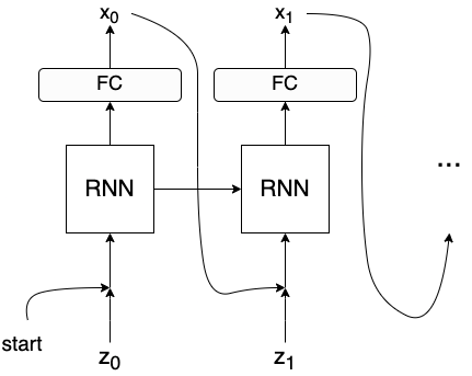
Note: In the paper, start is initialized from Uniform [-1, 1].
The discriminator is a bi-directional RNN followed by a fully connected layer.
The generator is implemented in PyTorch as follows,
RC-GAN
The next paper is ‘Real-Valued (Medical) Time Series Generation With Recurrent Conditional GANs’ (Esteban et al., 2017).
RC-GAN’s generator’s input consists of a sequence of latent variables.
The paper also introduces a ‘conditional’ GAN, where conditional/static information (\(c\)) is concatenated to the latent variables and used as input to improve training.
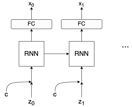
The discriminator is the same as in C-RNN-GAN but is not bi-directional.
The implementation is as follows,
Time-GAN
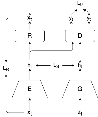
TimeGan (Yoon et al., 2019) is the most recent approach, which aims to maximize the similarities between embeddings of real data and fake data.
First, the generator (\(G\)) creates embeddings (\(\hat{h_t} = G(\hat{h_{t-1}}, z_t)\)) from latent variables while the embedding network (\(E\)) encodes real data (\(h_t = E(h_{t-1}, x_t)\)). The Discriminator (\(D\)) then discriminates between real and fake embeddings. While the Recovery network (\(R\)) reconstructs the real data (creating \(\hat{x_t}\)) from its respective embedding.
This leads to 3 losses
- Embedding difference (Goal: Similar embeddings for real and fake data)
Notice: \(G\) takes \(h_{t-1}\) as input, NOT \(\hat{h_{t-1}}\)
- Recovery Score (Goal: meaningful embeddings for real data)
- Discriminator Score
Note: Similar to the previous paper, the paper talks about static/context features which can be used throughout the training process (E.g the label (1, 2, …, 9) when generating the MNIST dataset). To simplify this post, I chose to sweep this little detail under the blogpost rug.
To complete the optimization, the total loss is weighed by two hyperparameters \(\lambda\) and \(\eta\) (whos values were found to be non-significant). Leading to the following…
\[\min_{E, R} \lambda L_S + L_R\] \[\min_{G} \eta L_S + \max_{D} L_U\]Empirical Results
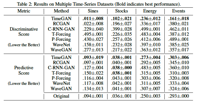
Below are the results comparing time-series focused, generative models. We can see that TimeGAN performs the best across all datasets with RC-GAN close behind. For a more detailed explanation of the data, refer to the paper.
RC-GAN + Stock Data
Since both RC-GAN and TimeGAN show similar results and RC-GAN is a much simpler approach we will implement and investigate RC-GAN.
Generator and Discriminator
Training Loop
Visualizing Stock Data
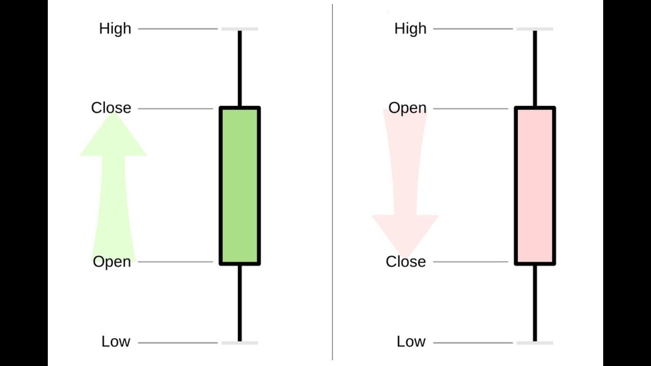
Before we generate stock data, we need to understand how stock data is visualized.
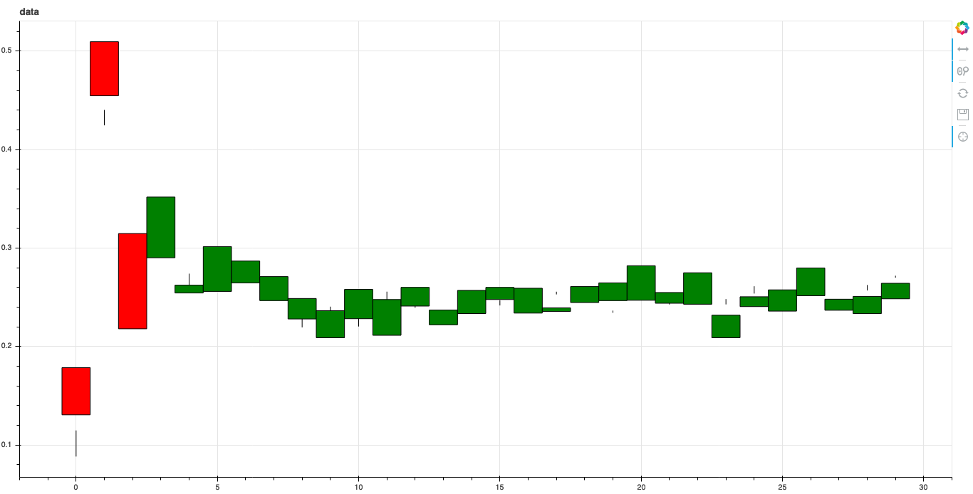
Every day, the price which the stock opened and closed at, and the highest and lowest price the stock reached that day is represented using a candlestick.
If the stock closed higher than it opened, the candle is filled green. If the stock closed lower than it opened, then the candle is filled red.
Nice!
Examples
The model was trained with the GOOGLE price data split into 30-day parts (used in the TimeGAN paper).
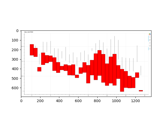
Below are some generated data along with low-dimension analysis using T-SNE.
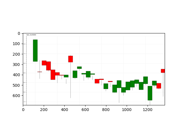
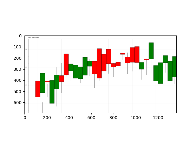
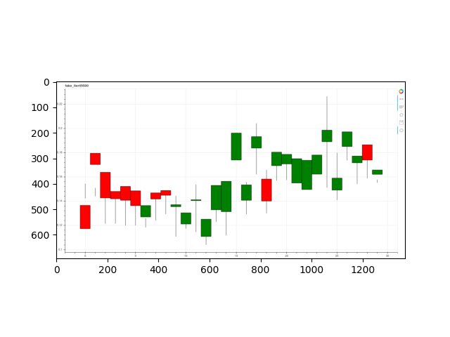
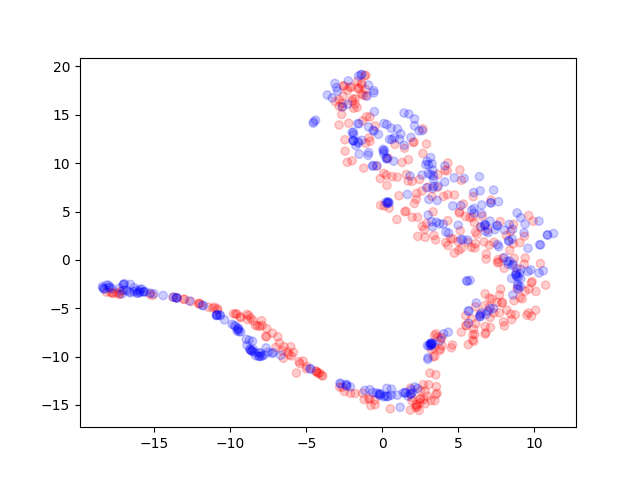
Though it looks that the examples overlap through a T-SNE visualization, they do not always look realistic.
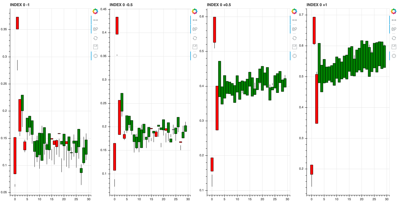
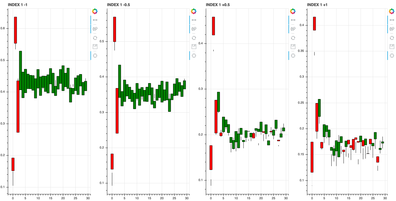
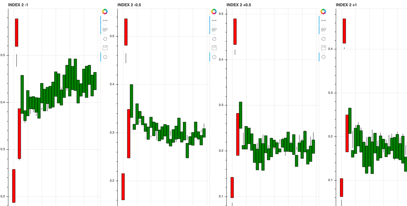
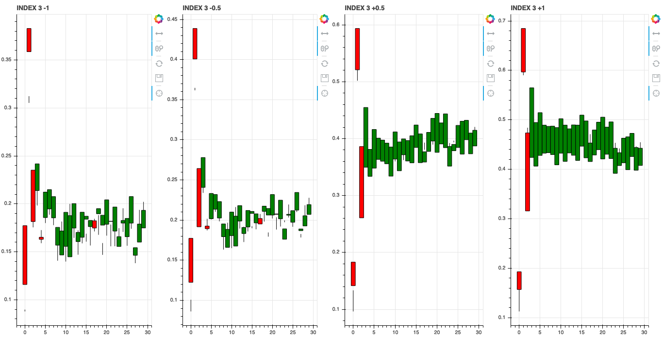
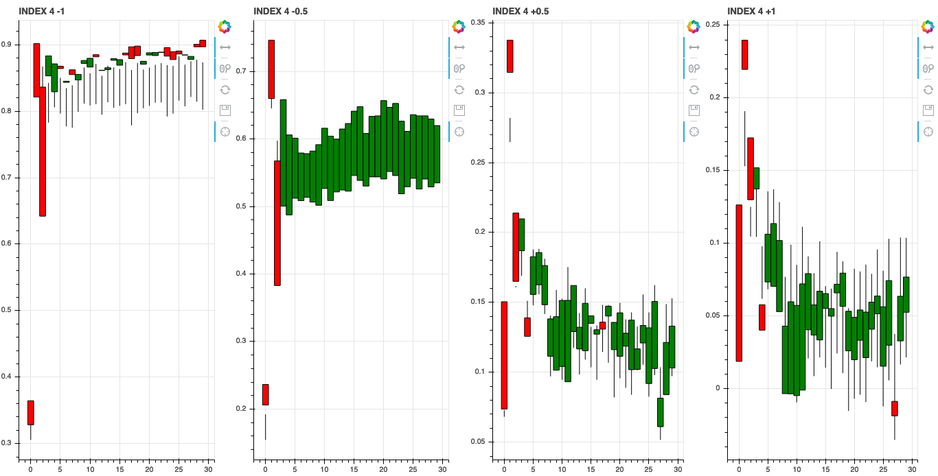
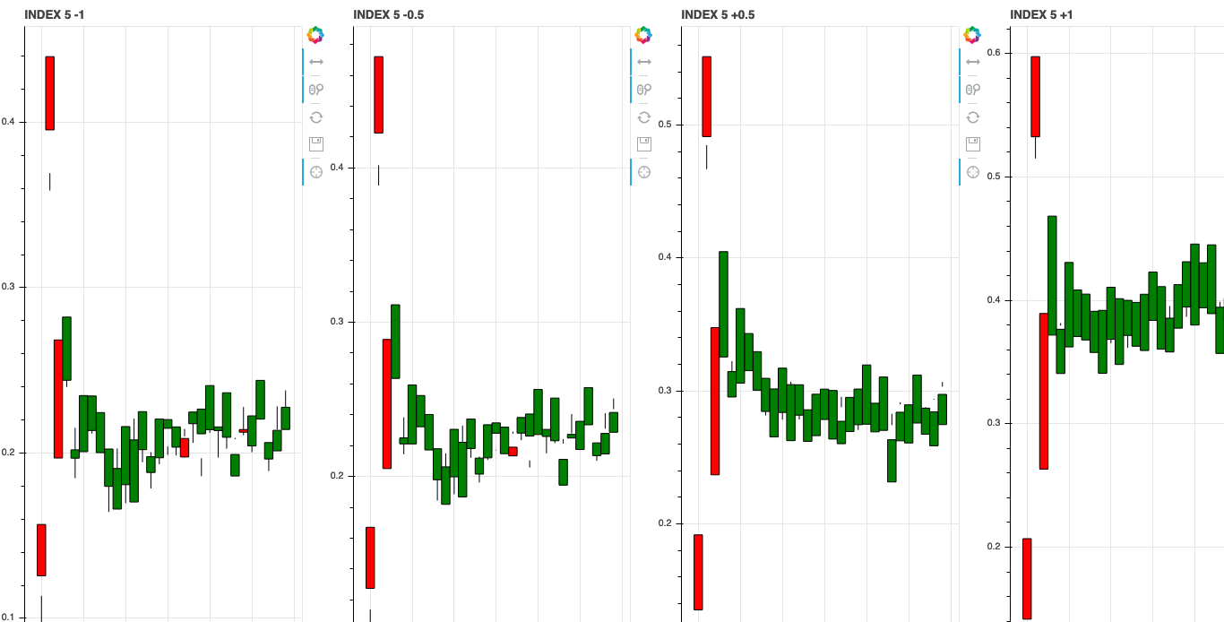
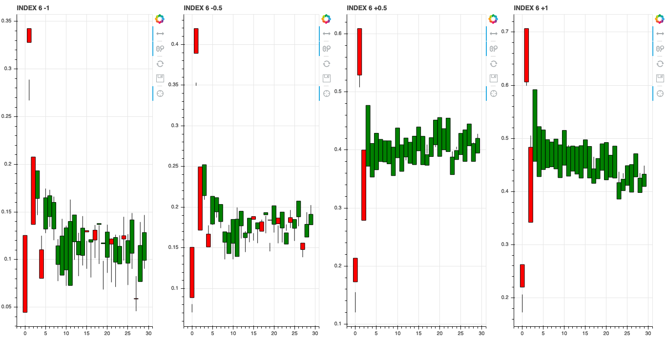
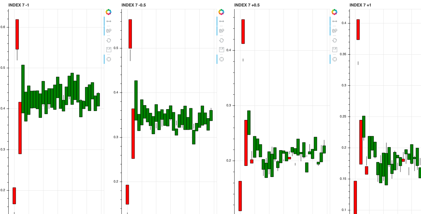
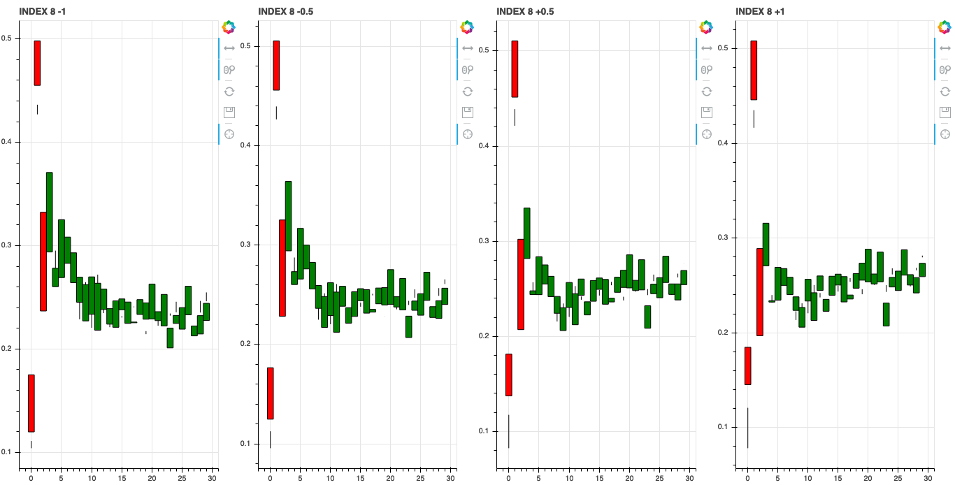
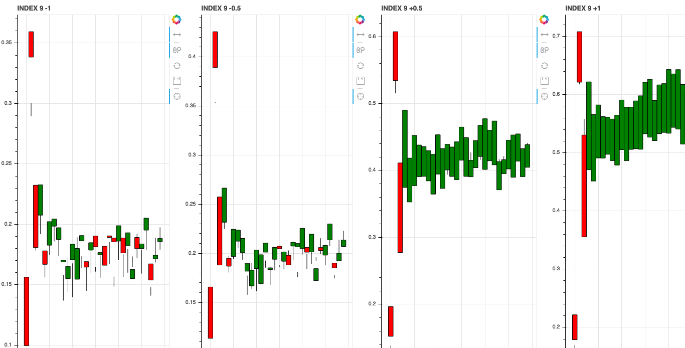
Feature Association
We can also investigate what the learned features associate with by shifting the axis values around in latent space. Since we trained our model with a \(z\) dimension of 10 we can shift the value of each of these dimensions and see how it changes the generated stock data.
[Original Generated Data]
Shifting Noise Axis Values [-1, -0.5, +0.5, +1]
Index 0
Index 1
Index 2
Index 3
Index 4
Index 5
Index 6
Index 7
Index 8
Index 9
There is also a notebook which contains all the code needed to test this out for yourself!
If you enjoyed the post, feel free to follow me on Twitter for updates on new posts!
References
- Mogren, O. (2016). C-RNN-GAN: Continuous recurrent neural networks with adversarial training. ArXiv Preprint ArXiv:1611.09904.
- Esteban, C., Hyland, S. L., & Rätsch, G. (2017). Real-valued (medical) time series generation with recurrent conditional gans. ArXiv Preprint ArXiv:1706.02633.
- Yoon, J., Jarrett, D., & van der Schaar, M. (2019). Time-series generative adversarial networks. Advances in Neural Information Processing Systems, 5508–5518.