Photo Link

When applying Convolutional Neural Networks (CNNs) (LeCun et al., 1990) to a computer vision task, a change in viewpoint (change in orientation, position, shear, etc.) is likely to lead to drastically different network activations, hindering the model’s ability to generalize. To solve this problem, current CNNs require a large number of parameters, datasets and computational power.

This lead to the introduction of Capsule Networks (Hinton et al., 2011). Capsule Networks aim to generalize to different viewpoints by taking advantage of the fact that the relationship between parts of an object is viewpoint invariant. It has been shown that these networks generalize better than standard CNNs, are more robust to adversarial attacks, achieve higher accuracy, all while requiring significantly fewer parameters.

In this post, we focus on the following topics…

• Introduction to the Viewpoint Problem
  • CNN’s Solution
  • Capsule Network’s Solution
• Introduction to Capsule Networks
• Routing Algorithms
  • Dynamic Routing Between Capsules (Sabour et al., 2017)
  • Matrix Capsules with EM Routing (Hinton et al., 2018)
    • with a prerequisite: Gaussian Mixtures with EM

Though this may seem intimidating, don’t worry, as long as you don’t have a medical phobia of capsules, you’ll be able to swallow all the knowledge in this post.

The Problem

The problem comes from the goal of computer vision generalization, as we want our models to generalize to unseen data. My version of generalization is as follows,

After training on an image, when tested on a slightly modified version of the image, the two responses are similar.

One of the main reasons that test images are ‘slight modifications’ of training images is a change in viewpoint. A change in viewpoint is defined as,

A change in the position from which something or someone is observed.

A few examples of viewpoint transformations are as follows,

• Rotations (rotating 90 degrees)
• Shifts (moving 30 pixels left)
• Scaling (zooming in/moving closer; shift in the +z axis)

Note: Viewpoint-transformations can modify part(s) of the image or the entire image and can be applied to any of the 3 dimensions (x, y, or z).

Tip: Would your model be able to identify the car throughout all of its different viewpoint changes?

If we can reasonably account for viewpoint variability in images we will improve model generalization. Consequently, when improving model generalization we are also likely to improve model test accuracy while requiring fewer data examples and parameters.

Solutions

In this section, we briefly discuss solutions to the change in viewpoint, including the CNN solution and The Capsule Network solution. Both solutions include some kind of representation learning and information routing.

We define activations as \(a \in A\), model input as \(x \in X\), our model as \(f: X \rightarrow A\) and a viewpoint transformation as \(T\).

The CNN Solution - Brute Force and Extract

To account for viewpoint changes, general CNNs aim to model viewpoint-invariance. Invariance is defined as,

\[f(Tx) = f(x) \tag{0}\]

Less formally, CNNs want their network activations to remain unchanged regardless of the viewpoint transformation applied. To show how CNNs could achieve this we must first introduce Data Augmentation and Max-pooling.

Data Augmentation - The Representations

A popular method to improve model generalization is to train on randomly augmented data examples. However, this turns out to be problematic and inefficient.

Learning viewpoint representations from data augmentations is difficult as most viewpoint transformations require 3D data. As most computer vision tasks train on 2D data, we are limited to simple 2D transformations.

Models which learn from the few viewpoint transformations we can apply turn out to be parameter inefficient. It’s been shown that early layers in a CNN trained with data augmentation are rotated, scaled and translated copies of one another (Zeiler & Fergus, 2013). This insight leads to the idea that CNNs could be learning specific feature detectors for each possible transformation to account for viewpoint variance, which is extremely inefficient.

Max-pooling - The Routing

Assuming that we have learned a feature detector for each corresponding viewpoint transformation, CNNs then attempt to route this information using the max-pooling layer (Riesenhuber & Poggio, 1999).

Max-pooling extracts the largest value in a group of neighbouring values.

\[f_{pool}: a_{pooled} = \max(a_{group}) \tag{1}\]

Max-pooling is locally shift-invariant because shifts which don’t move the largest value out of its group, result in the same \(a_{pooled}\) being extracted.

We can formulate the max-pooling invariance as the following,

\[f_{pool}( T_{localshift} x) = f_{pool}(x) \tag{2}\]

Applying max-pooling to feature maps of a network can help us learn a viewpoint-invariant model. For example, applying max-pooling to a group of rotation weight activations, we can extract the features of the best fit rotation. Doing so would allow us to become rotation invariant.

This leads to a CNNs approach to achieve viewpoint invariance; Learn a set of feature detectors for each viewpoint transformation and apply max-pooling to each group of transformation specific weights to extract/route the best fit activations.

However, an important problem with max-pooling is that we end up discarding a lot of useful information in the group.

Final Thoughts

In practice, it doesn’t work out nearly as nice and easy as I described but hopefully, this gives you a general idea about how representation learning and routing could be working with current CNNs.

Though this technique has lead to great results, it is easy to see how extremely inefficient and expensive to train a model like this is.

There must be a better way!

The Capsule Network Solution - A Capsule A Day Keeps The Invariance Away

Look no further, Capsule Network are here to save the day!

Unlike standard CNNs, Capsule Networks aim to model viewpoint-equivariance. Equivariance is defined as,

\[f(Tx) = Tf(x) \tag{3}\]

Less formally, Capsule Networks want their network activations to change in a structured way corresponding to the viewpoint transformation. The idea is that it would be easier to model complex distributions like images if our activations change in a structured way.

Capsule Networks achieve equivariance in two steps.

1. Explicitly represent parts located in the image.
2. Take advantage of the fact that the relationship between parts of an object is viewpoint invariant.

Assuming we can identify and represent simple parts in an image (step 1), it would be nice to be able to combine these simple parts to detect more complex objects.

For example, suppose we see the parts of an image are a pair of eyes, a nose and a mouth. Then I asked you, is there a face in the image? You would most likely check if the parts were structured in a certain way (eyes are above the nose, the mouth is right below the nose, etc.) and if they were, you would be confident there is a face in the image.

We can be confident there is a face in the image because there is a clear relationship between the eyes, the nose and the mouth to create a face. A great property about this relationship is that its viewpoint-invariant.

If we rotate, shift, change the brightness and apply a few other viewpoint transformations to the face (the object) and the relationships between the parts (the eyes, the nose and the mouth) and the object (the face) stay the same.

Tip: If you don’t believe me, look at your nose and move/rotate your head in any direction. If someone is watching you, your nose would be moving all over the place, but relative to your eyes, your nose won’t move at all. This is the invariance between parts of an object.

Capsule Networks work like this. We will dive more into the details next.

But before we do that, I ask you to repeat it with me…

‘What do we want?’

‘Equivariance to improve generalization requiring less data and parameters!’

‘When do we want it?’

‘Now!’

Excellent!

Introduction to Capsule Networks

In this section, we cover general details and the intuition behind Capsule Networks. For more posts on the topic see ‘More Resources’ at the bottom of the page.

We first define a few terms and the setup.

We refer to instances in an image as either a part or an object. The relationship is that a part belongs to an object. We assume a two-layer capsule network setup for conciseness. The first layer is referred to as low-level capsules (simple parts) and the second layer is referred to as high-level capsules (complex objects). Usually, the low-level capsules are known and we want to compute the high-level capsules. Don’t worry if that last part didn’t make sense, it will soon.

Part and Object Representations - The Part and The Capsule

1. Explicitly represent parts located in the image.

Learning to model parts of an image directly would be very difficult. This is because a simple viewpoint transformation results in a large difference in pixel space.

We want to learn a manifold where viewpoint transformations in pixel space result in simple and easy to model differences.

This manifold relates to the pose of a part (position, orientation, size), since applying a viewpoint transformation to the image would only result in a simple change to the affected part’s pose. Since this manifold would be very complex to specify, we learn it with a CNN.

Note: This is similar to learning a disentangled representation, which is a popular subject in generative modelling.

Note: A part could be represented by more than its pose. For example, we could represent a part by its velocity, albedo, or texture but for simplicity, we only consider its pose.

To extract capsules from the image we pass the image through the CNN and reshape it’s feature vectors to some \(H'\) x \(W'\) x \(CapsuleDim\). This aims to encapsulate parts of the image into the learned manifold.

Since we treat each section of the image as a part, we must also represent the probability that there is a part, which we refer to as the presence probability.

The vector which stores the pose and presence probability of a part is called a ‘capsule’.

Routing Information - Complex Objects

We now focus on how to combine detected parts to detect more complex objects, which is called ‘routing’.

2. Take advantage of the fact that the relationship between parts of an object is viewpoint invariant.

Since we represent parts and objects with pose matrices we can represent the relationship between a part’s pose and its corresponding object’s pose with a weight matrix. It’s important to remember that this weight would remain the same after applying any viewpoint transformation because the relationship is viewpoint invariant.

For example, given the pose of an eye \(p_{e}\), we can predict the corresponding face pose \(p_{f}\) as follows,

\[\begin{aligned} p_{e} \cdot W_{ef} &= p_{f} \\ \iff f(p_{e}) &= p_{f} \tag{4} \end{aligned}\]

Applying a transformation to the face object, by the viewpoint invariant relationship we get…

\[(T p_{e}) \cdot W_{ef} = T p_{f} \tag{5}\]

Rearranging and substituting we get,

\[f(T p_{e}) = T f(p_{e}) \tag{6}\]

Remind you of anything? Equivariance! \(f(T x) = T f(x)\). Since we are explicitly representing poses with network activations, our model will have viewpoint equivariance.

From simple parts extracted from the image, we now know how to detect more complex objects. But how can we be sure that the pose prediction is correct? and does the predicted face really exist?

Prediction Confidence - Agreement between Predictions

Think back to your early school days, back when you were given math homework. As readers of this blog, I’m sure you were/are all stellar students. Let’s assume your dog ate your finished homework and you can’t remember your answers.

Your teacher would never believe you! So you do what must be done. You cheat. I know, awful, it was tough to even type that out.

You go to your friends and ask them what answers they got. If they all got the same answer you can be pretty confident that answer is correct. However, if everyone got different answers then you cannot be sure which answer is correct.

We follow the same principles since we extracted multiple parts/low-level capsules (nose, ears, etc.) from the image, we ask them to predict the object/high-level capsules pose (face). We can set the high-level capsules pose as the most agreed upon prediction and its presence probability as the amount of agreement.

Example: If most low-level capsules agree on the high-level capsule’s pose, then we can be confident, by setting a high presence probability (activate the high-level capsule).

Usually, there will be more than one object represented in an image, so we repeat this process for every high-level capsule. Thus, every low-level capsule predicts every high-level capsule and we look for agreement between the predictions to set the high-level capsules’ value.

Capsule Recap

We achieve viewpoint equivariance by representing parts explicitly and taking advantage of the viewpoint invariant relationships between parts of an object.

We first transform the image into a manifold where viewpoint transformations result in simple changes, extracting poses and presence probabilities of parts in the image.

Each part (low-level capsule) predicts each object (high-level capsule). We route agreed-upon predictions to high-level capsules and set their presence probabilities as the amount of agreement between predictions.

Note: The number of low-level capsules can be related to the number of receptive fields in the eye (too few can result in ‘crowding’ where a single capsule/receptive field represents more than one part/object)

There are multiple ways to implement routing, we will cover two versions next.

Routing Algorithms

The two algorithms we will cover are ‘Dynamic routing between capsules’ and ‘Matrix Capsules with EM Routing’.

If you understood the intuition in the previous section then this should be a breeze.

Dynamic Routing Between Capsules

This paper implements a very standard and easy to understand version of Capsule Networks. We cover the high-level details, for more specific details refer to the paper or other posts in the ‘More Resources’ section.

Architecture

The network consists of the manifold CNN, a single layer of low-level capsules and a single layer of high-level capsules representing the classes of the classification task (10 classes/high-level capsules on MNIST).

The procedure is as follows

1. Extract low-level capsules using the CNN
2. Compute high-level capsules

Representations

The capsules are represented by 8-dimensional vectors and the presence probability is represented by the magnitude of the capsule. We extract features with a standard CNN and then reshape the features to produce capsules for our image.

Predictions

Low-level capsules predict high-level using weights \(W_{ij}\). The \(i^{th}\) low-level capsule predicts the \(j^{th}\) high-level capsule as \(\hat{u}_{j \mid i}\).

\[u_i \cdot W_{ij} = \hat{u}_{j\mid i} \tag{7}\]

Now that we know how to compute predictions for high-level capsules, we focus on how to computationally find agreement.

Routing with Agreement

For each \(j^{th}\) high-level capsule, we will have \(I\) predictions (\(\hat{u}_{1 \mid j}, \hat{u}_{2 \mid j}, ..., \hat{u}_{I \mid j}\)), one from each of the \(I\) low-level capsules.

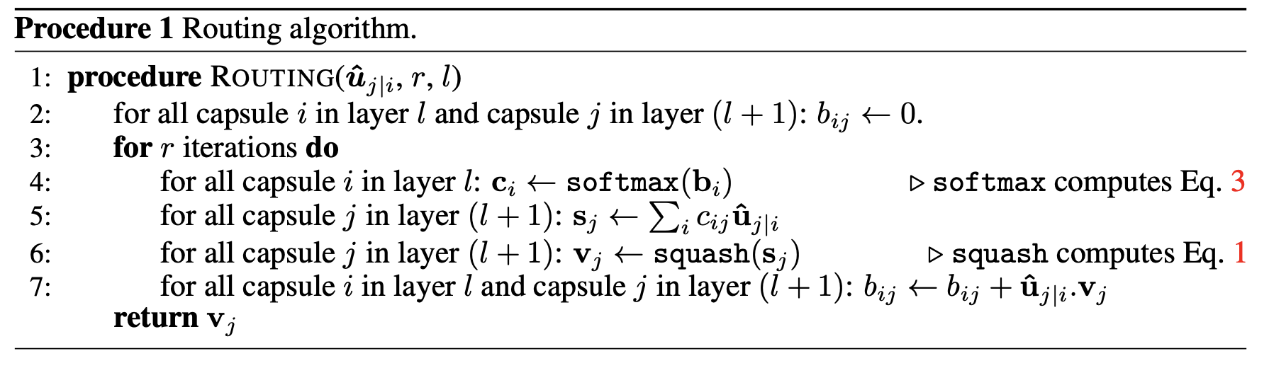
We find agreement with an iterative algorithm which consists of three steps,

1. Compute the high-level capsule \(s_j\), with a linear combination of predictions
2. Apply the squash function to \(s_j\)
3. Increase the weight of inlier predictions

First we assign routing weights for each of the \(K\) predictions, \(c_{1 \mid j}, c_{2 \mid j}, ..., c_{I \mid j}\) for every \(j^{th}\) capsule. They are all initialized to zero.

\[\underline{Iteration Start}\]

To ensure that each part corresponds to a single object, we apply the softmax to each low-level capsules routing weights.

\[c_i = softmax(c_i) \tag{8}\]

For each high-level capsule, we compute the high-level pose \(s_j\) with a linear combination of predictions weighted by the routing weights from the low-level capsules.

\[s_j = \sum_i c_{i \mid j} \hat{u}_{i \mid j} \tag{9}\]

The squash function is then applied to ensure \(\|\mathbf{v_j}\| \leq 1\).

\[v_j = \dfrac{\|\mathbf{s_j}\|^2}{1 + \|\mathbf{s_j}\|^2} \dfrac{s_j}{\|\mathbf{s_j}\|} \tag{10}\]

Next, we update the weights \(c_{i \mid j}\) by how much they ‘agree’ with the predicted \(v_j\). Where the dot is vector dot product.

\[c_{i \mid j} = c_{i \mid j} + (\hat{u}_{i \mid j} \cdot v_j) \tag{11}\]

Since \(\hat{u}_{i \mid j} \cdot v_j = \|\mathbf{\hat{u}_{i \mid j}}\| \|\mathbf{v_j}\| \cos \theta\) where \(\theta\) is the angle between the two vectors. Since \(\cos \theta\) has a maximum value when \(\theta = 0\) we end up increasing the weight of vectors whos angle is close to \(v_j\).

\[\underline{Iteration End}\]

In practice, we repeat the iteration 3-5 times to find agreement.

Note: This is similar to finding a cluster centroid in the predictions.

That is all we will cover since there are a lot of great resources online covering this algorithm. Taken from the paper, the algorithm is below.

Matrix Capsules with EM Routing Prereq.

The next algorithm we will cover is ‘Matrix Routing with EM’. Since this algorithm is the most complex and least covered online, we will focus on it in-depth.

The algorithm relies on Gaussian Mixtures and Expectation-Maximization. We will review both topics and how they relate to the main algorithm.

If you are familiar with both feel free to jump to the ‘Matrix Capsules with EM Routing’ section which begins to review the paper.

For more detailed explanations and derivations on Gaussian Mixtures and EM, I highly suggest you read the linked Mixture Models notes written by University of Toronto faculty.

Mixture of Gaussian

For an awesome additional resource on this topic checkout Roger Grosse’s notes here

Modeling

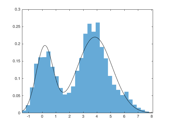
Assume our data distribution is multimodal (more than one hump). We would like to model our data with the efficient Gaussian distribution but a single Gaussian would not fit the data well.

What in the world shall we do? The data world has not been kind to us but as readers of this blog, we will not go quietly in the night. We shall do the unthinkable and model our data with a mixture of MULTIPLE Gaussians!

For generality, assume we want to model our data with \(K\) Gaussian distributions and our data consists of \(N\) points.

Modelling our data with multiple Gaussians we can derive the likelihood as follows,

\[\begin{aligned} p(x) &= \sum_K P(x | z=k) \; p(z=k) \\ &= \sum_K \pi_k \; P(x | z=k) \tag{12}\\ &= \sum_K \pi_k \; \mathcal{N}(x \mid \mu_k, \sigma_k) \\ \end{aligned}\]

So the parameters we aim to optimize \(\theta = \{\mu_1, \sigma_1, \pi_1, ..., \mu_K, \sigma_K, \pi_K\}\)

Optimizing with Expectation-Maximization

There are multiple ways we could optimize our model but we do not settle for just any technique. You got it, we focus on expectation-maximization! An elegant and efficient algorithm for optimizing model parameters to our data.

Note: There is a more general form of EM which applies to any latent distribution but since we only use the Gaussian mixture edition, we will only focus on it.

The heart of the algorithm is the following formula,

\[\begin{aligned} \dfrac{d}{d\theta}\log{p(x)} &= \mathbb{E}_{p(z\mid x)}[\dfrac{d}{d\theta} \log p(z, x)] \tag{13} \\ &= \mathbb{E}_{p(z\mid x)}[\dfrac{d}{d\theta} \log p(z) + \log p(x \mid z)] \\ \end{aligned}\]

Computing \(\log p(z)\) and \(\log p(x \mid z)\) is trivial since \(\log p(z)\) is a learned parameter \(\pi_k\) and \(\log p(x \mid z)\) can be calculated with the Gaussian PDF formula.

How would we compute \(p(z\mid x)\)? We use bayes rule to get,

\[\begin{aligned} p(z \mid x) &\propto p(x \mid z) p(z) \tag{14}\\ \\[0.2mm] p(z=k \mid x) &= \dfrac{p(x \mid z=k) p(z=k)}{\sum_K p(x \mid z=k) p(z=k)} \\ \\[0.2mm] &= \dfrac{\pi_k \mathcal{N}(x \mid \mu_k, \sigma_k)}{\sum_K \pi_k \mathcal{N}(x \mid \mu_k, \sigma_k)} \end{aligned}\]

Now that we know how to compute every term, out of curiosity we evaluate the log-likelihood’s derivative \(d \ell\) for our parameters \(\mu_k\), \(\sigma_k\) and \(\pi_k\)

For simplicity we let \(r_k^{(i)} = p(z = k \mid x^{(i)}) = \dfrac{\pi_k \mathcal{N}(x^{(i)} \mid \mu_k, \sigma_k)}{\sum_K \pi_k \mathcal{N}(x^{(i)} \mid \mu_k, \sigma_k)}\).

Solving for the derivative of the mean of the \(k^{th}\) Gaussian, \(\mu_k\)

\[\begin{aligned} \dfrac{d \ell}{d\mu_k} &= \mathbb{E}_{p(z\mid x)}[\dfrac{d}{d\mu_k} \log p(z) + \log p(x \mid z)] \\ &= \sum_{i=1}^{N} r_k^{(i)} \; [\dfrac{d}{d\mu_k} (\log p(z = k) + \log p(x^{(i)} \mid z = k))] \quad \text{[By definition of Expectation]}\tag{15}\\ &= \sum_{i=1}^{N} r_k^{(i)} \; [\dfrac{d}{d\mu_k} (\log \pi_k + \log \mathcal{N}(x^{(i)} \mid \mu_k, \sigma_k))] \\ &= \sum_{i=1}^{N} r_k^{(i)} \; \dfrac{d}{d\mu_k} \log \mathcal{N}(x^{(i)} \mid \mu_k, \sigma_k) \\ &= \sum_{i=1}^{N} r_k^{(i)} \; (0 + \dfrac{x^{(i)} - \mu_k}{\sigma_k^2}) \\ &= \sum_{i=1}^{N} r_k^{(i)} \; \dfrac{x^{(i)} - \mu_k}{\sigma_k^2} \\ \end{aligned}\]

This looks very simple, so simple we should be able to solve for the optimal value by setting the derivative to zero. Doing so we get the optimal value \(\mu_k^*\),

\[\mu_k^* = \dfrac{\sum_{i=1}^{N} r_k^{(i)} x^{(i)}}{\sum_{i=1}^{N} r_k^{(i)}} \tag{16}\]

Bystander: Whoa there cowboy, your \(r_k\) depends on \(\mu_k\) and thus that optimal value is incorrect. You should put on this approximate hat to signify you it is not the true optimal value…

\[\hat{\mu}^*\]

Though this is not the true optimal value, it turns out to be a good approximation. This approximated optimal parameter \(\hat{\mu_k}^*\) is used as a ‘step’ towards the true optimal parameter \(\mu_k^*\).

We can derive similar results on the other parameters by fixing \(r_k^{(i)}\) to obtain approximate optimal values \(\hat{\theta}^*\) for parameters \(\theta\).

\[\hat{\pi_k}^* \leftarrow \dfrac{1}{N} \sum_{i=1}^N r_k^{(i)} \tag{17}\\ \\[0.4cm] \hat{\mu_k}^* \leftarrow \dfrac{\sum_{i=1}^N r_k^{(i)} x^{(i)}}{\sum_{i=1}^N r_k^{(i)}} \\[0.4cm] \hat{(\sigma_k^2)}^* \leftarrow \dfrac{\sum_{i=1}^N r_k^{(i)} (x^{(i)} - \mu_k)^2}{\sum_{i=1}^N r_k^{(i)}}\]

This leads us to the iterative EM algorithm

The \(E\)-Step: Compute responsibilities \(r_k\).

\[r_k^{(i)} \leftarrow p(z = k \mid x^{(i)}) \tag{18}\]

The \(M\)-Step: Compute and update parameters \(\theta\) to the approximate optimal parameters \(\hat{\theta}^*\)

\[\theta \leftarrow \arg\max_{\theta} \sum_{i=1}^N \sum_{k=1}^K r_k^{(i)} [\log p(z=k) + \log p(x^{(i)} \mid z = k)] \tag{19}\]

The algorithm fits our data iteratively by

1. Increase/decrease the weights \(r_k\) to the best/worst fit distributions
2. Update the parameters to fit the current weights

Does this sound familiar? If you flip the steps and let the brain work its magic you have something similar to the Dynamic Routing algorithm.

In the next section, we talk about how we can use this algorithm to model capsule routing and agreement with a Gaussian distribution.

Matrix Capsules with EM Routing

We can now introduce EM Routing. The goal is to model low-level capsule votes with a multi-dimensional Gaussian. This turns out to be very similar to EM with a mixture of Gaussians.

Representations

A capsule is represented by a 4x4 pose matrix \(M\) and an activation probability \(a\). Therefore, each capsule will have dimensions (4 x 4 + 1).

We extract the first level capsules by passing the image through the CNN and then reshaping it’s features to some \(H'\) x \(W'\) x (4 x 4 + 1).

Predictions

The \(i^{th}\) low-level capsule makes predictions for the \(j^{th}\) high-level capsules with a learned 4x4 matrix \(W_{ij}\). There is a slight change in notation in the paper, so we will use the updated paper’s notation for consistency.

Where \(u_i \cdot W_{ij} = \hat{u}_{j\mid i}\) is changed to \(M_i \cdot W_{ij} = V_{ij}\) in the paper. \(V_{ij}\) is the \(i^{th}\) low-level capsule’s ‘vote’ for the \(j^{th}\) high-level capsule. As well, the routing weights \(c_{i \mid j}\) are now referred to as \(R_{ij}\).

Routing

The main difference in this algorithm is how routing is conducted.

For the \(j^{th}\) high-level capsule we have \(I\) low-level capsule predictions (\(V_{1j}, V_{2j}, ..., V_{Ij}\)).

We refer to the capsules in the \(L^{th}\) layer as \(\Omega_L\)

The low-level capsules are the known capsules (usually \(\Omega_L\)) and the high-level capsules, are the capsules we are computing (usually \(\Omega_{L+1}\)).

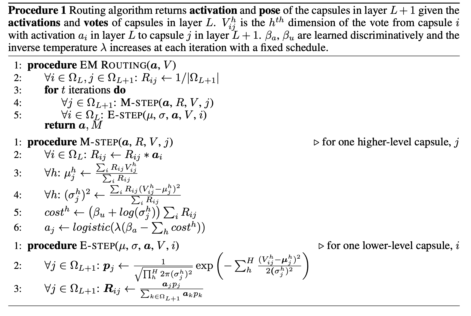
First, we initialize the low-level capsules routing weights uniformly across the high-level capsules

\[\forall i \in \Omega_L, j \in \Omega_{L+1}: R_{ij} \leftarrow \dfrac{1}{\mid \Omega_{L+1} \mid} \tag{20}\]

We then iterate between a \(M\)-step for each high-level capsule and an \(E\)-step for each low-level capsule.

\[\underline{Iteration Start}\\ \\[5mm] \forall j \in \Omega_{L+1}: \text{M-STEP}(\textbf{a}, R, V, j)\]

The \(M\) step is as follows,

1. Since we only care about the votes for existing parts and active capsules, we re-weight the routing weights by each low-level capsule’s presence probability.

   \[\forall i \in \Omega_L: R_{ij} \leftarrow R_{ij} * a_i \tag{21}\]

2. We then use EM to solve for the approximate optimal parameters for the Gaussian over the low-level capsule votes.

   Note: Since the votes \(V_{ij}\) are multidimensional, we have to compute parameters for each dimension \(h\).

   \[\forall h: \mu^h_j \leftarrow \dfrac{\sum_i R_{ij} V_{ij}^h}{\sum_i R_{ij}} \tag{22}\\ \\[0.4cm] \forall h: (\sigma_j^h)^2 \leftarrow \dfrac{\sum_i R_{ij} (V_{ij}^h - \mu_j^h)^2}{\sum_i R_{ij}}\]

3. We now focus on how to compute the high-level capsule’s presence probability \(a_j\). Following the intuition of, if there is agreement between votes then the high-level capsule should be present. We can compute the ‘agreement’ by how well the Gaussian fits the weighted votes using its probability density function (PDF).

   Computing the pdf \(P_{i \mid j}^h\) of the \(i^{th}\) low-level capsule’s vote under the \(j^{th}\) high-level capsule’s Gaussian’s \(h^{th}\) component is as follows,

   \[P_{i \mid j}^h = \dfrac{1}{\sqrt{2\pi(\sigma_j^h)^2}} \exp(-\dfrac{(V_{ij}^h - \mu_j^h)^2}{2(\sigma_j^h)^2}) \tag{23} \\ \\[0.4cm] \ln(P_{i \mid j}^h) = -\dfrac{(V_{ij}^h - \mu_j^h)^2}{2(\sigma_j^h)^2} - \ln(\sigma_j^h) - \ln(2\pi)/2\]

   Taking into account the routing weights, the total \(Agreement\) on the \(h^{th}\) component of the \(j^{th}\) high-level capsule is as follows,

   \[{Agreement}_j^h = \sum_i R_{ij} \ln(P_{i \mid j}^h) \tag{24}\]

   We want to maximize agreement. In the paper, instead of agreement they refer to the cost (negative agreement). Minimizing the cost is the same as maximizing the agreement. We can simplify the cost equation of a high-level capsule is as follows,

   \[\begin{aligned} {cost}_j^h &= \sum_i -R_{ij} \ln(P_{i \mid j}^h) \\ &= \dfrac{\sum_i R_{ij} (V_{ij}^h - \mu_j^h)^2}{2(\sigma_j^h)^2} + (\ln(\sigma_j^h) + \dfrac{\ln{(2\pi)}}{2})\sum_i R_{ij} \\\tag{25} \\[0.1mm] &= \dfrac{\sum_i R_{ij} (V_{ij}^h - \mu_j^h)^2}{2(\dfrac{\sum_i R_{ij} (V_{ij}^h - \mu_j^h)^2}{\sum_i R_{ij}})} + (\ln(\sigma_j^h) + \dfrac{\ln{(2\pi)}}{2})\sum_i R_{ij} \quad \text{[By definition of } (\sigma_j^h)^2 \text{]}\\ \\[0.1mm] &= \dfrac{1}{2} \sum_i R_{ij} + (\ln(\sigma_j^h) + \dfrac{\ln{(2\pi)}}{2})\sum_i R_{ij} \\ &= (\ln(\sigma_j^h) + \dfrac{1}{2} + \dfrac{\ln{(2\pi)}}{2})\sum_i R_{ij} \end{aligned}\]

   This equation ends up being the standard deviation weighted by the total amount of information flowing into the capsule. We thus want to find tight agreement in the votes to minimize the standard deviation, \(\sigma_j^h\) resulting in low cost. We compute the cost as follows,

   \[cost^h \leftarrow (\beta_u + \log(\sigma_j^h)) \sum_i R_{ij} \tag{26}\]

   Note: \(\beta_u\) is a learned parameter. This offers the model more flexibility instead of directly using the other constant terms (\(\dfrac{1}{2} + \dfrac{\ln{(2\pi)}}{2}\)) in the derived equation.

   Since we either activate the capsule or don’t, we need to define the minimum value of agreement required to activate. Another way of saying this is, we need a maximum value of cost so that exceeding this cost, we don’t activate the capsule. We do so with the following formula,

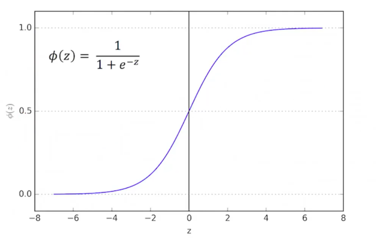
   \[a_j \leftarrow logistic(\lambda(\beta_a - \sum_h cost^h)) \tag{27}\]

   This equation means that the cost of an activated capsule must be less than \(\beta_a\), where \(\beta_a\) is a learned parameter.

   Since when we begin training our predictions will be very random, we use \(\lambda\) (an inverse temperature parameter) as a way to be less strict to capsule activations to allow gradients to flow. We increase the strictness throughout the training process as our predictions become more accurate.

   The logistic function either activates the capsule or not depending on if its value is larger than some threshold.

   

And that is the \(M\) step in full detail. We compute the approximate optimal parameters of the Gaussian over the low-level capsule votes and evaluate the standard deviation of the Gaussian to decide whether or not to activate the high-level capsule.

Next, we cover the simpler \(E\)-step. This step updates the weights \(R_{ij}\) by how well they agree with the high-level Gaussian.

The \(E\)-step is as follows,

\[\forall i \in \Omega_L: \text{E-STEP}(\mu, \sigma, \textbf{a}, V, i)\]

1. We first compute how well the votes agree under the high-level capsule.

   \[\forall j \in \Omega_{L+1}: p_j \leftarrow \dfrac{1}{\sqrt{\prod_h 2\pi(\sigma_j^h)^2}} \exp(- \sum_h \dfrac{(V_{ij}^h - \mu_j^h)^2}{2(\sigma_j^h)^2}) \tag{28}\]

2. We then compute the routing weights as \(a_jp_j\) and normalize so all routing weights from a single low-level capsule sum to one.

   \[\forall j \in \Omega_{L+1}: R_{ij} \leftarrow \dfrac{a_jp_j}{\sum_{k \in \Omega_{L+1}} a_kp_k}\tag{29}\]

Notice how computing \(R_{ij}\) is the same as computing the responsibilities \(r_k^{(i)}\). We first compute \(p(x \mid z)\) as \(p_j\) and \(p(z)\) as \(a_j\) and then normalize to satisfy bayes rule. We only modify how we compute \(a_j\).

\[\underline{Iteration End}\]

At the end of the iterations, we use \(a_j\) as the presence probability and \(\mathbf{\mu_j}\) as the pose for the high-level capsule.

And that’s Matrix Capsules with EM Routing’s algorithm! Taken from the paper, the algorithm is below.

Recap

We covered EM with a mixture of Gaussian and understood how to achieve routing with such an algorithm by fitting a gaussian to the votes.

We first covered the \(M\) step where we solve for the approximate optimal parameters of a Gaussian under the low-level capsules votes and decide whether to activate the high-level capsule depending on if there is enough agreement between the votes. We then covered the E-step, where we recompute the routing weights depending on how well the vote falls under the high-level Gaussian.

The Future of Capsule Networks

Why have they not been able to achieve state of the art?

Unfortunately, the current hardware is not optimized to run these kinds of algorithms at scale (Barham & Isard, 2019).

Conclusion

We first covered the viewpoint problem which hinders computer vision model generalization. We then investigated how CNNs and Capsule Networks approach the viewpoint variance problem. Lastly, we covered the general intuition of Capsule Networks and two different routing algorithms.

Thanks for reading!

Let me know what you think about the post below!

If you want more content? Follow me on Twitter!

References

1. LeCun, Y., Boser, B. E., Denker, J. S., Henderson, D., Howard, R. E., Hubbard, W. E., & Jackel, L. D. (1990). Handwritten Digit Recognition with a Back-Propagation Network. In D. S. Touretzky (Ed.), Advances in Neural Information Processing Systems 2 (pp. 396–404). Morgan-Kaufmann. http://papers.nips.cc/paper/293-handwritten-digit-recognition-with-a-back-propagation-network.pdf
2. Hinton, G. E., Krizhevsky, A., & Wang, S. D. (2011). Transforming Auto-Encoders.
3. Sabour, S., Frosst, N., & Hinton, G. E. (2017). Dynamic Routing Between Capsules.
4. Hinton, G. E., Sabour, S., & Frosst, N. (2018). Matrix Capsules With EM Routing.
5. Zeiler, M. D., & Fergus, R. (2013). Visualizing and Understanding Convolutional Networks.
6. Riesenhuber, M., & Poggio, T. (1999). Hierarchical models of object recognition in cortex.
7. Barham, P., & Isard, M. (2019). Machine Learning Systems are Stuck in a Rut.

More Resources

• Dynamic Routing Capsule Network Video Tutorial: https://www.youtube.com/watch?v=pPN8d0E3900

• Geoffrey Hinton Capsule Network Talk (2019): https://www.youtube.com/watch?v=x5Vxk9twXlE

• EM Routing Blog Post with TF Code: https://jhui.github.io/2017/11/14/Matrix-Capsules-with-EM-routing-Capsule-Network/

• Gaussian Mixture Models in PyTorch Blog Post: https://angusturner.github.io/generative_models/2017/11/03/pytorch-gaussian-mixture-model.html